Executive Summary
Portfolio optimization replaces manual security selection with a rules-based, automated process that improves outcomes and handles complex constraints. This whitepaper explains how institutional investors can apply optimization to sharpen decisions and simplify portfolio management.
Optimization tools manage constraints, run fast scenario analyses, and surface opportunities that manual methods often miss. They’re especially effective for portfolios with requirements like liability matching, credit guidelines, and regulatory limits.
Through a real-world case study, we show how optimization helps portfolio teams assess trade-offs, make defensible decisions, and measure the cost of constraints while staying aligned with governance standards.
A Primer in Portfolio Optimization
Optimization finds the best solution to a problem within predefined limits. In optimization terms, we use “objective function” and “constraints” to describe these two aspects. The optimizer aims to either maximize or minimize the objective function.
For example, imagine a postman delivering mail. He tries to minimize delivery time (objective) while delivering all the mail (constraint).
Formally:

Finding a solution can be a creative process. Different methods can be used, affecting both solution quality and computation time. Portfolio managers often approach the same problem differently. One might maximize returns with environmentally friendly investments, while another integrates specific research insights.
Optimization and Numerical Methods
Once the problem is defined, the optimizer can consider various methodologies for reaching a solution. Some methods are thorough but slower, while others are faster but might miss potential solutions. The “best” method depends on the problem.
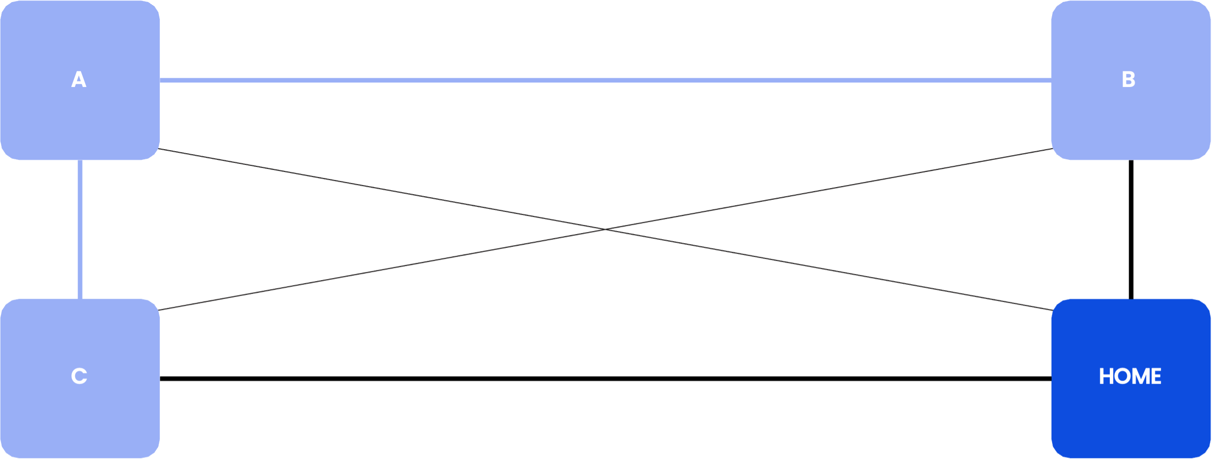
Consider our postman who must visit three houses: A, B, and C. Vertical paths take 6 minutes, horizontal ones 8 minutes, and diagonal ones 10 minutes.
We can list all possible solutions and select the one that minimizes overall time:
| Path | Time (minutes) |
| Home – A – B – C – Home | 36 (10 + 8 + 10 + 8) |
| Home – A – C – B – Home | 32 (10 + 6 + 10 + 6) |
| Home – B – A – C – Home | 28 (6 + 8 + 6 + 8) |
| Home – B – C – A – Home | 32 (6 + 10 + 6 + 10) |
| Home – C – A – B – Home | 28 (6 + 8 + 6 + 8) |
| Home – C – B – A – Home | 36 (10 + 8 + 10 + 8) |
The optimal solutions are Home – B – A – C – Home or Home – C – A – B – Home.
This demonstrates two key concepts:
- The optimization solution isn’t always unique
- Exploring all scenarios can be impractical, thus requiring more sophisticated methods
For example, we could note that taking diagonal paths are never efficient and should only explore paths without them:
| Path | Time (minutes) |
| Home – B – A – C – Home | 28 (6 + 8 + 6 + 8) |
| Home – C – A – B – Home | 28 (6 + 8 + 6 + 8) |
The results coincide with the solutions found above.
Portfolio managers should consider the problem’s nature and choose methods that balance efficiency and accuracy. Sometimes finding a “good enough” solution quickly is better than spending valuable time searching for the perfect solution.
Portfolio Optimization: Asset Allocation vs. Security Selection
Portfolio optimization commonly refers to two distinct applications: asset allocation and security selection.
Asset allocation distributes portfolios across asset classes. Security selection chooses individual securities within an asset class to achieve investment objectives defined in the investment policy statement (IPS). We’ll briefly cover both but focus primarily on security selection.
Asset allocation can include broad classes (fixed income, equities, commodities) or more detailed divisions (sectors, geography). This typically uses mean-variance optimization (MVO) where portfolio risk and return are determined by measured return, variance, and covariance of asset classes. The optimal portfolio maximizes return while satisfying risk tolerances and investment objectives. For example, risk-tolerant policies might favor equities, while risk-averse approaches may lean toward fixed income.
Security selection identifies specific assets within allocated asset classes. Both processes work together to achieve investment objectives. This paper assumes asset allocation and IPS are established. We will be focusing on managing portfolio positions, specifically fixed-income security selection by a state government
While these optimization concepts provide the foundation, real-world implementation requires specialized tools. Portfolio managers face daily decisions involving hundreds of securities and complex constraints — challenges that exceed what manual spreadsheets can handle. Effective optimization demands reliable data integration, repeatable processes, and the ability to evaluate scenarios quickly while maintaining compliance.
Portfolio Optimizer Solutions
Transitioning from theory to practice requires effective tools. A portfolio optimizer enables users to input existing portfolios and investable universes, configure objective functions, and specify constraints. The software then generates an optimized solution while meeting requirements that maximize or minimize the chosen objective.
Note: Screenshots in this paper reflect Clearwater Wilshire’s current desktop Portfolio Optimizer. An enhanced web-based interface will be available in H2 2025.
Process Automation
The first step is reliably streamlining data intake for the investable universe. A model is only as good as its input data, which should meet the following criteria:
- Accuracy: Free from errors and reflecting true values
- Timeliness: Relates to present circumstances
- Relevance: Pertinent to the decision at hand
- Completeness: Including all necessary information to avoid partial or skewed understanding
Process automation is crucial to meeting these requirements. Manual data processing makes it difficult to maintain accuracy, completeness, and relevance. A key feature of a good portfolio optimizer is integration with existing data systems.
The second challenge is repeatability. Portfolio optimization is an ongoing process that managers must replicate for auditing and keeping investment decisions current. Monitoring, trading, and auditing require automation, so analysts can focus on optimization parameters and results, rather than manually reviewing each step as they would with spreadsheets.
A portfolio optimizer enables more efficient and reliable decision-making for any organization investing cash —including asset managers, insurance companies, government entities, and corporations.
Decision-Making vs. Black Boxes
Investment decisions require balancing mathematical optimization with portfolio manager judgment. Portfolio optimizers solve problems systematically — they satisfy constraints and find portfolios that maximize/minimize the objective function without second-guessing. This is especially true for point-in-time optimization without scenario projections. As objective functions become more complex and algorithms more sophisticated, understanding the optimizer’s steps becomes harder, risking “black box” decision-making.
Since portfolio managers are accountable for their decisions during audits and downturns, they cannot rely solely on optimizer outputs. When reviewing solutions, effective managers will:
- Check for unusual securities and verify underlying data
- Evaluate trade sizes for practicality
- Estimate transaction costs
- Identify constraints that limit the solution
- Consider how relaxing constraints might affect outcomes
- Assess solution stability over time
This questioning helps build a narrative around the solution that satisfies stakeholders and bolsters decision-making. The case study below illustrates this reasoning.
Case Study: Optimization in Action
To demonstrate how portfolio optimization works in practice, we’ll examine a real-world case study of a U.S. state government that used Clearwater’s optimizer to improve their portfolio performance. This analysis will show:
- How to set up an optimization problem
- The importance of well-designed constraints
- How to evaluate and interpret optimization results
- The financial impact of differing constraint choices
We start with a portfolio of short-term U.S. treasuries and use a separate portfolio of broker offerings as the investable universe (constructed from the Wilshire Gov/Corp index).
Vanilla Yield Optimization
![]()
Running the optimizer without constraints on our opportunity set produces an underwhelming result. The entire portfolio value is invested in the highest-yielding security available. This creates a highly concentrated portfolio with a lower credit rating and a different duration. This approach hardly requires specialized software but demonstrates how linear optimizers work and why well-designed constraints matter. The optimizer is rigid with a goal that does not consider practical limitations unless explicitly specified.
State Government Use Case
This real-world case involves a U.S. state government managing public funds. It needs to meet operational obligations while avoiding significant credit or currency risk. It prefers keeping existing investments and focuses on investing in available cash to maximize yield.
These constraints can be challenging to navigate daily without the proper infrastructure. Optimizers that handle these constraints while accurately integrating data are invaluable in such situations. Trading securities is a common process, and portfolio optimizers add significant efficiency.
- Investable universe: Available securities to purchase (e.g. USD fixed income securities)
- Constraints: Set of conditions to be met by the solution portfolio (e.g. only investment-grade securities)
Once defined, the portfolio optimizer will take care of data integration and solution finding.
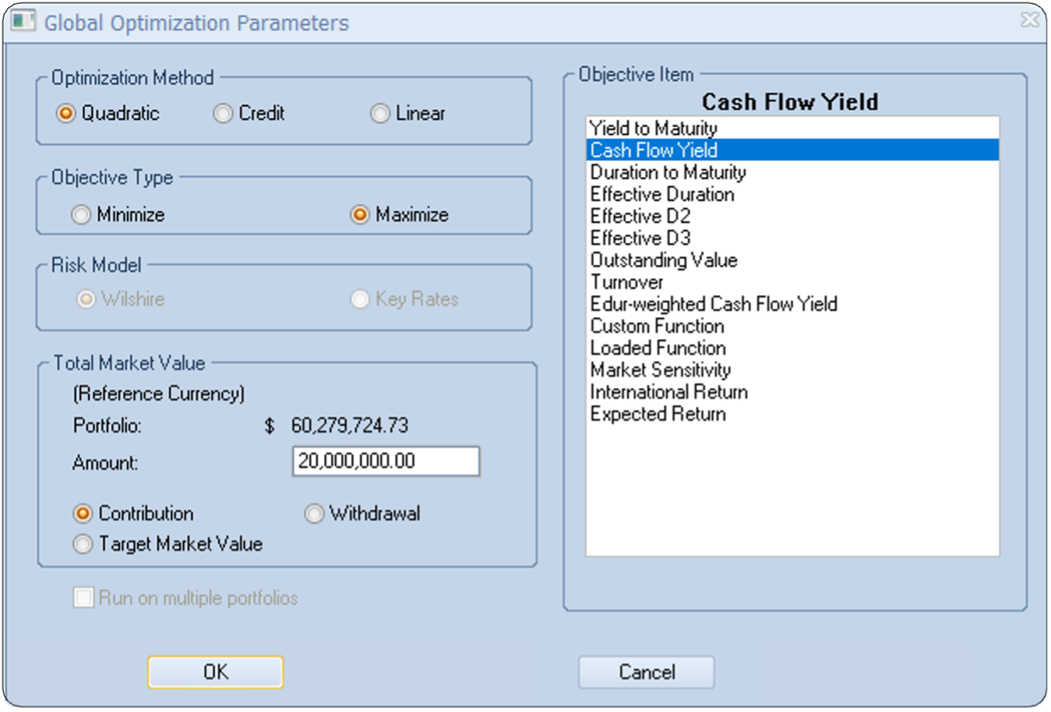
In this case, we load existing holdings, specify available cash ($20M), and define the objective function (maximize cash flow yield). We enable “Specify Liability to Match” since this government must meet defined liabilities.
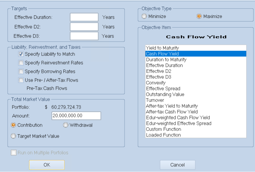
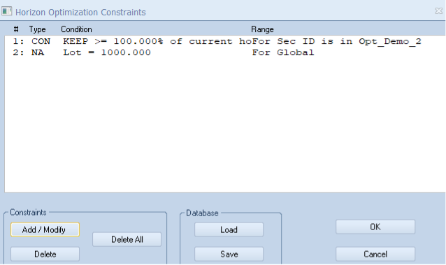
We set these constraints:
- Investments must be from the defined investable universe (OPT_DEMO_1), containing only USD securities
- Securities must be investment grade according to Moody’s rating

- Current portfolio securities (OPT_DEMO_2) cannot be sold
- Purchases should be in 1,000-unit lots
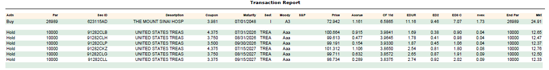
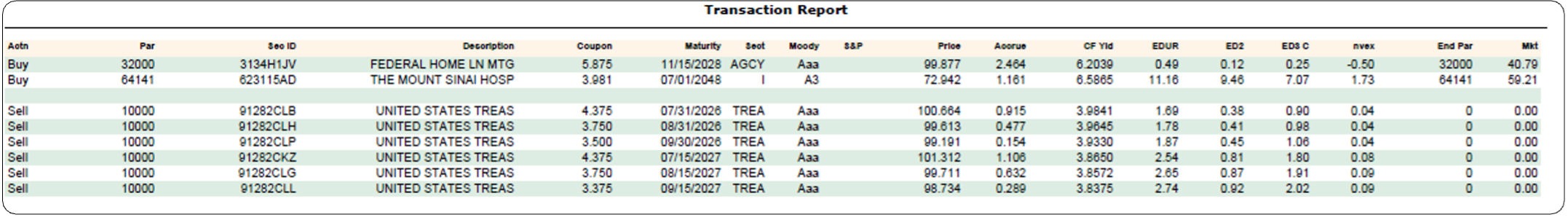
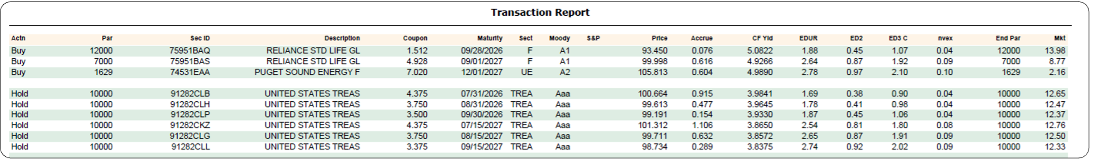
The solution provides several reports:
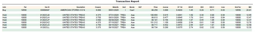
- Transaction Report: Shows actions (hold/sell) on existing securities and new purchases, with key features like maturity date, price, duration, and convexity
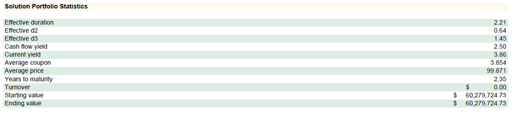
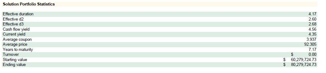
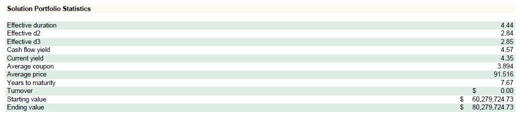
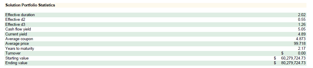
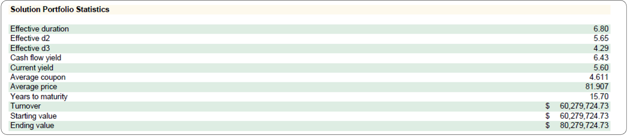
- Portfolio Statistics: Compares solution statistics like duration and yield with the starting portfolio
- Constraint Report: Summarizes whether the optimizer met all constraints
- Liability Matching: Shows solution portfolio cash flows against liabilities
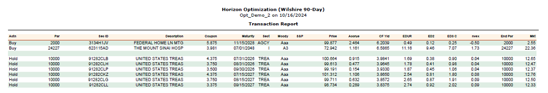
The last six rows show existing assets with “hold” action, as requested. The optimizer suggests buying two new securities:
- Security 1: Purchase 2,000 units (meeting the 1,000 multiple requirement) of AAA-rated bond with high yield, maturing in 2028
- Security 2: Purchase larger quantity of AAA-rated bond with slightly higher yield, maturing in the distant future
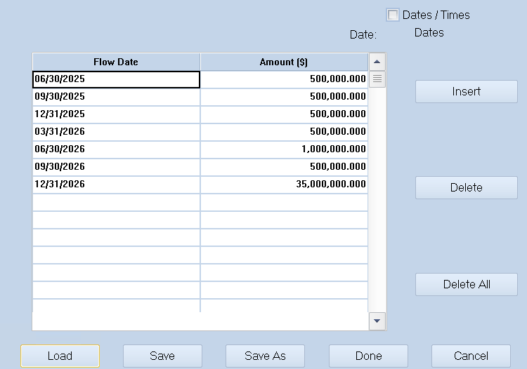
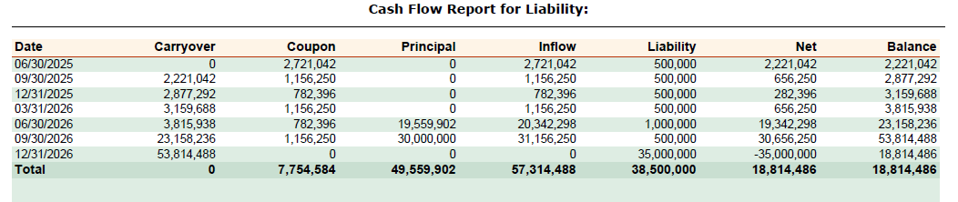
To verify liability coverage, we check portfolio cash flows:
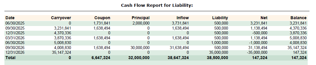
The balance column remains positive for all liability dates, satisfying the constraints. The final balance is small, which is appropriate since maximizing yield requires minimizing uninvested cash.
Note the first row shows principal payment in 2025, though no securities mature that year. Investigation reveals security 3134H1JV has a callable feature expected to be exercised on April 1, 2025. This demonstrates how the optimizer interacts with security modeling to project cash flows accurately.
The major principal payment in late 2026 comes from three maturing securities in the current portfolio. These inflows, with previous payments, provide sufficient cash for the large final liability.
The solution portfolio improves yield from 3.91% to 4.56%, a 65bps increase:
Relaxing Constraints
Relaxing or removing one constraint at a time allows us to investigate their costs. Here we outline the various combinations of constraints removal along with the resulting portfolios and final yields.
Here are the main constraints:
- Liability constraint: Meet the given liabilities
- Rating constraint: Invest only in investment-grade securities
- No selling constraint: Use only available cash to purchase new securities and do not sell the securities in the current portfolio
Let’s review the results of removing one or more of these constraints at a time:
- Constraints relaxed: The constraints removed before each run of the optimizer
- Current securities: Whether to sell or hold the securities in the current portfolio
- Purchase securities: The securities to purchase from the investable universe
- Final yield: The cash flow yield of the solution portfolio
| Constraints relaxed | Current securities | Purchase securities | Final yield |
| Initial Position | Hold | NA | 3.91% |
| None (base case) | Hold | Federal Home (AAA, 6.20%) Mount Sinai (A3, 6.59%) | 4.56% |
| No liabilities | Hold | Mount Sinai (A3, 6.59%) | 4.57% |
| No ratings | Hold | American Stores (Caa1, 8.49%) | 5.05% |
| Allow selling | Sell all securities | Federal Home (AAA, 6.20%) Mount Sinai (A3, 6.59%) | 6.43% |
| No liabilities, no ratings | Hold | American Stores (Caa1, 8.49%) | 5.05% |
| No liabilities, allow selling | Sell all securities | Mount Sinai (A3, 6.59%) | 6.59% |
| No ratings, allow selling | Sell all securities | American Stores (Caa1, 8.49%) | 8.49% |
| Fully unconstrained | Sell all securities | American Stores (Caa1, 8.49%) | 8.49% |
The Federal Home security is needed to meet the liability constraint, and the rest of the cash is invested into the Mount Sinai security, which provides a higher yield while satisfying the Investment-grade constraint.
Remove the Liabilities Constraint
Without liability constraints, the optimizer no longer purchases Federal Home and invests all cash in Mount Sinai. The yield increases to 4.57%, just 1 basis point higher than the base case—a very low constraint cost.
This provides useful insight: The optimizer abandons the AAA-rated Federal Home security for just 1 basis point of yield. Portfolio managers must evaluate whether concentrating so heavily in Mount Sinai is appropriate despite the optimizer’s mathematical preference.
Portfolio statistics after removing liability constraints:
Remove the Credit Rating Constraint
Without credit rating constraints, the optimizer seeks higher yields regardless of credit quality. This directs all available cash to a riskier security, American Stores (Caa1 rating, 8.49% yield), which nearly doubles the current portfolio yield. This security matures in June 2026, meeting liability needs.
The yield increases from 4.56% to 5.05% – a constraint cost of about 0.5% compared to the base case.
Portfolio & key statistics after removing credit rating constraints:
Remove the “Hold” Constraint
Removing the restriction on selling existing assets lets the optimizer sell all current securities to buy higher- yielding ones while respecting other constraints. This creates a portfolio with more Federal Home securities to help meet liabilities:
The liability coverage with the new portfolio:
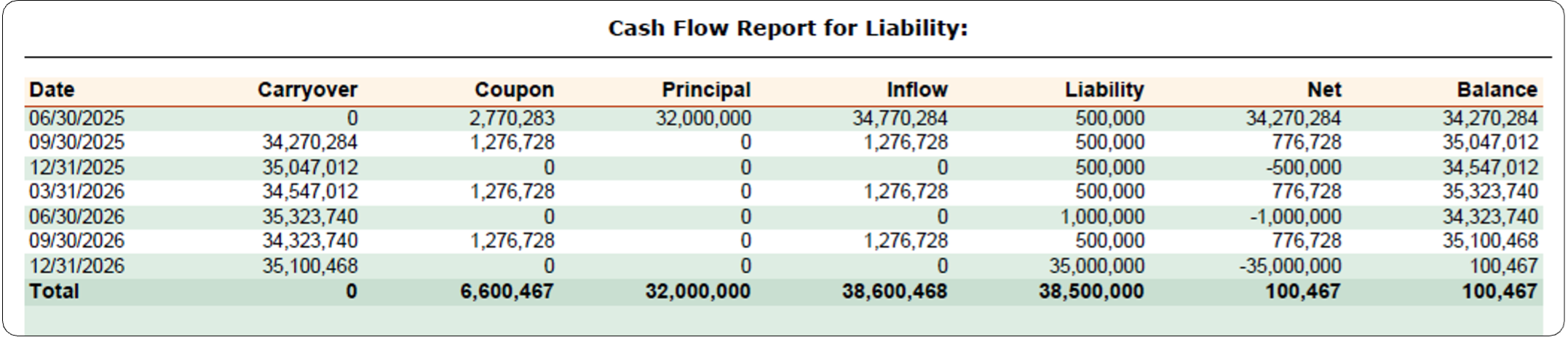
Relaxing the selling constraint has the greatest impact, increasing yield from 4.56% to 6.43%– a constraint cost of 1.87%:
Changing Optimization Method
Let’s introduce another parameter by minimizing the tracking error from the initial portfolio. This means building a portfolio that:
- Respects the constraints
- Maximizes the cash flow yield
- Has characteristics which are not too dissimilar from the initial one
For simplicity, we’ll remove liability constraints and keep only the rating constraint, lot size constraint, and no-selling constraint.
This problem requires a quadratic method that can minimize tracking error while maximizing yield:
The option is selected as follows:
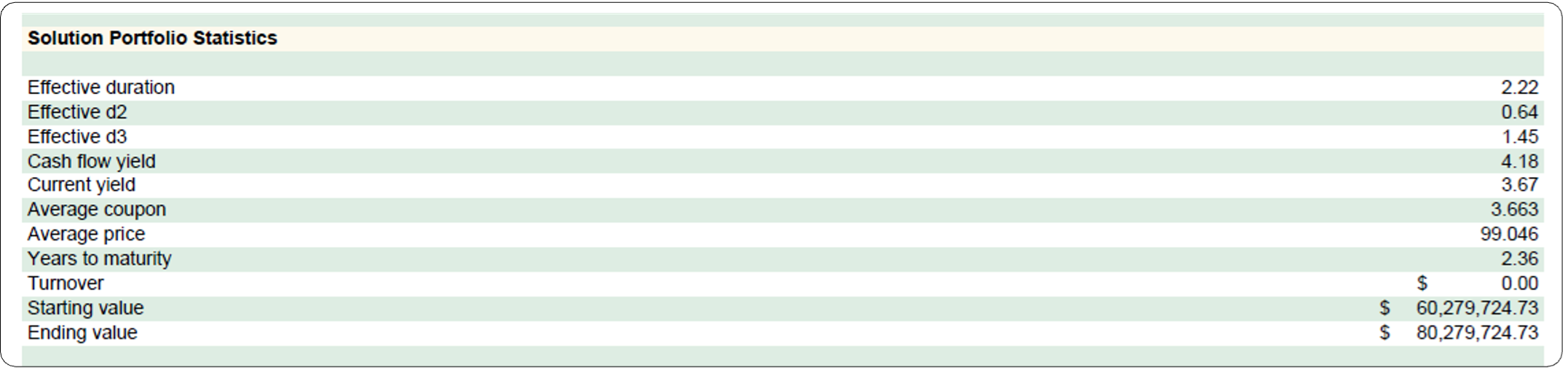
The purchased securities have similar duration and convexity to the initial portfolio but lower ratings (still investment grade), yielding 4.18% versus the initial 3.67%. The linear solver, which didn’t consider the tracking error, produced a higher yield of 4.57%. This demonstrates how adding constraints reduces optimization freedom.
Conclusion
Efficient portfolio optimization improves financial returns by:
- Streamlining data for identifying investable universes
- Automatically screening securities to meet constraints
- Finding securities that optimize objectives while satisfying constraints
The objective function should reflect the institution’s specific needs. In our case study, the goal was maximizing yield while meeting credit rating and liability constraints.
Appendix A details various portfolio manager use cases. Managers should question and adjust constraints to find better solutions. Our case study showed the benefits of relaxing constraints – information that can inform investment committee reviews. In short, managers should question and adjust constraints to find better solutions.
Portfolio managers relying solely on spreadsheets may miss opportunities that optimizers can identify. Appendix B covers daily challenges, from transaction costs to model limitations.
Portfolio optimization combines the objective with the subjective and evolves through dialogue and situational analysis rather than a set of fixed truths.
Appendix A: Portfolio Optimizer Use Cases
Yield Maximization
Return maximization is a primary objective for many portfolios. Yield maximization seeks securities with the highest possible return based on yield measures. For fixed income, these include yield to maturity, current yield, and yield to call, each offering different insights.
In this paper, yield maximization refers to cash flow yield – yield based on likely security cash flows, incorporating optionality and prepayment. This approach assumes a constant yield curve throughout security life.
Yield maximization becomes practical when combined with constraints. Without constraints, optimizers focus solely on yield at the expense of credit risk, liquidity, etc. For example, illiquid, low-coupon, long-maturity securities might be selected for investors with short-term liquidity needs. Best practice involves balancing yield maximization with constraints on credit ratings, duration, transaction costs, etc. Investors should understand yield trade-offs when adding constraints.
Cost of Constraints
Yield maximization provides a starting point for identifying attractive investments. An unconstrained yield-maximized portfolio establishes a benchmark for the highest attainable yield.
Each constraint added either reduces yield or has minimal effect. Quantifying these “constraint costs” helps investors make informed decisions. For example, restricting to investment-grade bonds might reduce yield from 8% to 6%, a 200 basis point constraint cost. Geographic restrictions might have minimal cost if similar-risk bonds exist in the preferred regions.
Understanding constraint costs helps investors balance risk and return, evaluate whether constraints are necessary, and explain how regulatory requirements affect returns. This analysis is critical for making informed decisions and achieving tailored investment objectives.
Liability matching
The final use case we will cover is liability matching — timing cash flows to meet known future obligations. Consider a family managing monthly bills with the following simplified payment schedule:
They need liquidity on specific dates but don’t need to hold all cash year-round. For example, they don’t need to keep the $12,000 for annual taxes in cash throughout the year—they could invest that money safely and liquidate the needed portion at the beginning of April each year. Similarly, since their monthly expenses amount to $1,200, they could invest in bonds providing monthly coupons of $1,200 to meet liabilities while preserving capital.
Financial institutions face similar challenges with added complexity, particularly those with highly predictable cash flows. Pension funds exemplify this approach, especially those offering defined benefit plans. They know with some level of certainty when account holders will retire and how much they’ll need to pay on a recurring basis, enabling strategic investment planning.
Effective liability matching meets obligations through portfolio cash flows (coupons and dividends) rather than asset sales, reducing transaction costs and risks. This approach also benefits credit ratings: by consistently meeting liabilities, financial institutions demonstrate lower default probability to investors. Detailed approaches like accounting defeasance are beyond this paper’s scope.
Portfolio optimizers excel at liability matching by analyzing cash flow timing, selecting securities that generate payments when needed, and balancing yield optimization with liquidity constraints while maintaining capital preservation.
Appendix B: Challenges & Pain Points
Portfolio management involves implicit constraints and costs that impact investment returns. A common question arises: “If these cannot be explicitly described in a portfolio optimizer, how can I account for them in the optimization process?”
Liquidity
Liquidity presents multiple challenges in portfolio optimization. Consider when an optimizer suggests selling a large position in an existing security to purchase one better suited for the objective function. If the security to be sold is illiquid, several problems arise: selling takes time while the target security’s price may rise, or forced quick sales occur below market price, reducing purchasing power for the replacement security.
Liquidity is critical for liability matching. Liabilities can be met through portfolio cash flows (coupons, dividends, maturities) or asset sales. Since liabilities must be met promptly, any assets earmarked for sale must be sufficiently liquid.
Capturing liquidity dynamics in optimizers is challenging since liquidity has no concrete parameter and fluctuates over time.
Three approaches address this:
- Pre-select an investable universe containing only sufficiently liquid securities
- Rate securities’ liquidity and use these ratings as penalties in the objective function
- Constrain the minimum cash that must be always held in the portfolio
Liquidity also significantly affects transaction costs.
Transaction costs
Transaction costs are among the most difficult aspects to capture in optimization since they’re not directly observable in input data and depend on factors like brokers used and market conditions. Often overlooked, transaction costs can cause portfolio managers to underperform benchmark indices.
Transaction costs increase with trade size — something optimizers examining only data typically miss. Adding penalties in the objective function that increase with purchase size might address this, but implementation proves difficult. Transaction costs are hard to measure and estimate, making penalty parameter tuning potentially impossible.
While difficult to measure, transaction costs always exist. One approach to reduce them in optimization setup involves modifying current portfolio data. For yield maximization objectives, add a few basis points to each existing security’s yield, encouraging the optimizer to avoid selling these positions.
An in-depth examination of transaction costs can be found in Grinold, Kahn-Active Portfolio Management: A Quantitative Approach for Producing Superior Returns and Controlling Risk-McGraw-Hill (1999).
Model limitations
Model quality depends on data quality—the “Garbage In, Garbage Out” principle. Poor input data cannot produce meaningful output.
Consider the simple optimization model run on a security universe made only of bonds:

Imagine the security universe to be made by the following data:
| Security | Credit rating | Annual yield |
| Safe&Secure Company | AAA | 2% |
| The Stable Company | AAA | 2.2% |
| Reliable Progress Org | AA | 3% |
| Junk & Co | AA | 12% |
The optimizer would purchase all available Junk & Co bonds since they meet the stated constraints. However, any financial analyst would immediately flag that a 12% annual yield is suspicious for an AA-rated bond. This yield suggests either a lower credit rating or incorrect yield data.
When the analyst investigates, they discover Junk & Co actually has a CCC rating. This disqualifies the security from the optimization since the constraint requires credit quality above AA.
When dealing with complex securities like options and derivatives, model choice and quality significantly impact solutions. Analysts must understand the models used, examining not just expected values but return distributions and sensitivities to market variables and parameters.
The complexity of modeled securities increases these challenges. Portfolio managers should critically analyze models before accepting solutions, understanding both capabilities and limitations.
Investment Policy Statement (IPS) Constraints
Beyond investment mandates and benchmarks, most investors face explicit constraints agreed upon with clients or principals. These constraints are diverse but may include:
- Investable universe limitations: Restrictions on self-dealing, asset class or sector allocations, geographic restrictions
- Portfolio risk controls: Limits on liquidity, position sizes, diversification requirements
- Investment strategy requirements: Sector neutrality relative to benchmark, exclusion of short positions
Constraints are important to integrate early in portfolio construction as they often pull portfolios away from theoretically optimal unconstrained solutions. Understanding these limitations helps portfolio managers balance compliance requirements with performance objectives.
References and Sources
- Grinold, Kahn-Active Portfolio Management: A Quantitative Approach for Producing Superior Returns and Controlling Risk-McGraw-Hill (1999)
- Catherin Ehrlich, Lawrence Berger: Asset Liability Modeling and Portfolio Optimization Seminar (1997)
- Harry Markovitz: Portfolio Selection: Efficient Diversification of Investments (1959)
- Harry Markovitz: Portfolio Selection, the Journal of Finance (1952)
- Owen Concannon, CFA, Robert M. Conroy, DBA, CFA, Alistair Byrne, PhD, CFA, and Vahan Janjigian, PhD, CFA: Portfolio Management section of the CFA Curriculum 2024
- Investopedia, https://www.investopedia.com/
©2025 Clearwater Analytics. All rights reserved. This material is for information purposes only. Clearwater makes no warranties, express or implied, in this summary. All technologies described herein are registered trademarks of their respective owners in the United States and/or other countries. 1/25